Week 1
Model selection with an AI assistance
Based on the AI’s suggestion, SVM is initially selected as the model for the research implementation.
Dataset: SMS Spam Collection Task: Text Classification
Load the dataset
Show/Hide the code
| |
| label | message | |
|---|---|---|
| 0 | ham | Go until jurong point, crazy.. Available only ... |
| 1 | ham | Ok lar... Joking wif u oni... |
| 2 | spam | Free entry in 2 a wkly comp to win FA Cup fina... |
| 3 | ham | U dun say so early hor... U c already then say... |
| 4 | ham | Nah I don't think he goes to usf, he lives aro... |
| ... | ... | ... |
| 5567 | spam | This is the 2nd time we have tried 2 contact u... |
| 5568 | ham | Will ü b going to esplanade fr home? |
| 5569 | ham | Pity, * was in mood for that. So...any other s... |
| 5570 | ham | The guy did some bitching but I acted like i'd... |
| 5571 | ham | Rofl. Its true to its name |
5572 rows × 2 columns
Data Preparation
Show/Hide the code
| |
Dummy Model
Show/Hide the code
| |
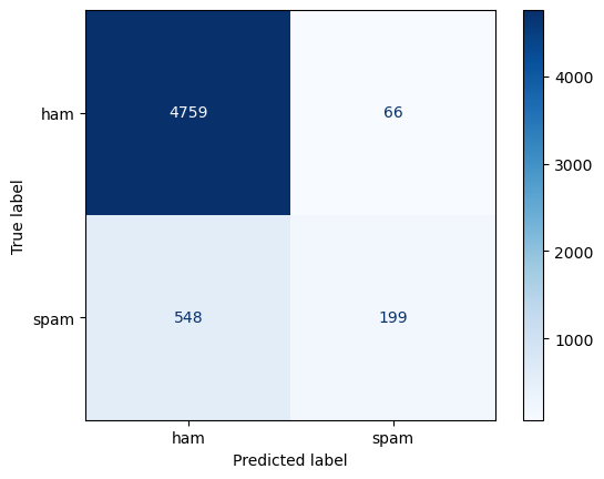
The result shows that this dummy model an extremely low recall, reflecting its inability to detect spam messages.
Show/Hide the code
| |
Accuracy: 0.8898061737257718
Precision: 0.7509433962264151
Recall: 0.26639892904953144
F1 Score: 0.3932806324110672

Classification Report:

              precision    recall  f1-score   support

         ham       0.90      0.99      0.94      4825
        spam       0.75      0.27      0.39       747

    accuracy                           0.89      5572
   macro avg       0.82      0.63      0.67      5572
weighted avg       0.88      0.89      0.87      5572
The confusion matrix
Show/Hide the code
| |
Week 2
SVM is a type of linear classifier. Its simplest form is the maximum margin classifier. This kind of classifier requires the data to be linearly separable and seeks an optimal hyperplane to divide the data into two classes. The criterion for finding the optimal hyperplane is that it should be as far away from the data points as possible. In order to understand the concepts of data points, hyperplanes, and their relationships with the basic machine learning framework — Hypothesis, Loss, and Optimizer — I decided to first implement a perceptron classifier and study its learning process
Perceptron Learning Algorithm
The implementation of a Perceptron Classifier.
A perceptron classifies data using a hyperplane defined by a linear function $f(x) = w \cdot x + b$. It has been proven that if the data is linearly separable, the perceptron algorithm is guaranteed to converge. Let the class label be denoted by $y$, where $y = 1$ for the positive class and $y = -1$ for the negative class. The predicted label is given by $\hat{y} = \text{sign}(f(x))$, and the product $\hat{y}y$ indicates the correctness of the prediction: a positive value implies a correct prediction, while a negative value indicates a misclassification.
When a data point is correctly classified, the algorithm proceeds to the next data point without updating the model. However, in the case of a misclassification, the model parameters are updated according to the following rules:
$$ w \leftarrow w + y \cdot x \cdot \text{lr} $$$$ b \leftarrow b + y \cdot \text{lr} $$where $\text{lr}$ is the learning rate that pre-defined by human.
This update mechanism implies that if the true label is positive, the normal vector $w$ of the hyperplane is adjusted in the direction of $x$, thereby increasing the likelihood of correctly classifying $x$ as a positive instance. Conversely, if the true label is negative, the vector $w$ is updated in the opposite direction of $x$, making it more likely that $x$ will be classified as negative.
If the dataset is linearly separable, the perceptron algorithm will converge to a solution in a finite number of steps. Otherwise, it will continue to update indefinitely without convergence.
The code below implements a simple perceptron classifier according to above descriptions, with an ability to record training processing.
Show/Hide the code
| |
Show/Hide the code
| |
Generate some mock data
Show/Hide the code
| |
Show/Hide the code
| |
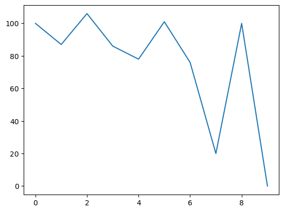
100
87
106
86
78
101
76
20
100
0
loss
Show/Hide the code
| |
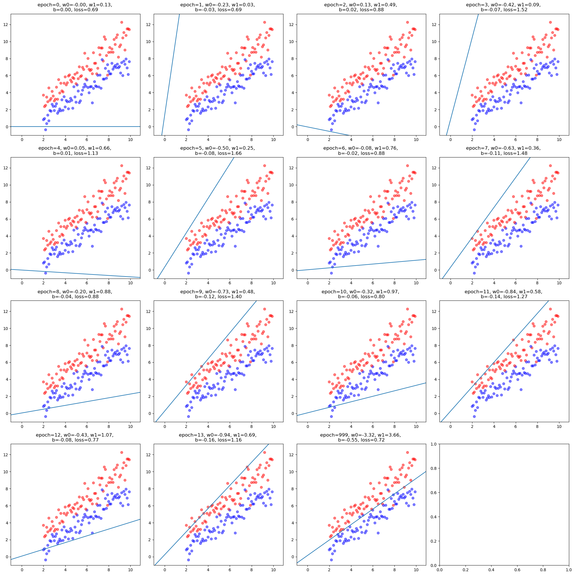
Visualize the hyperplane
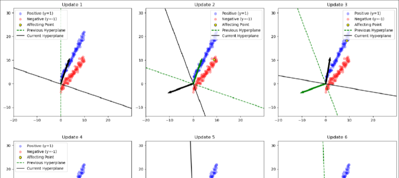
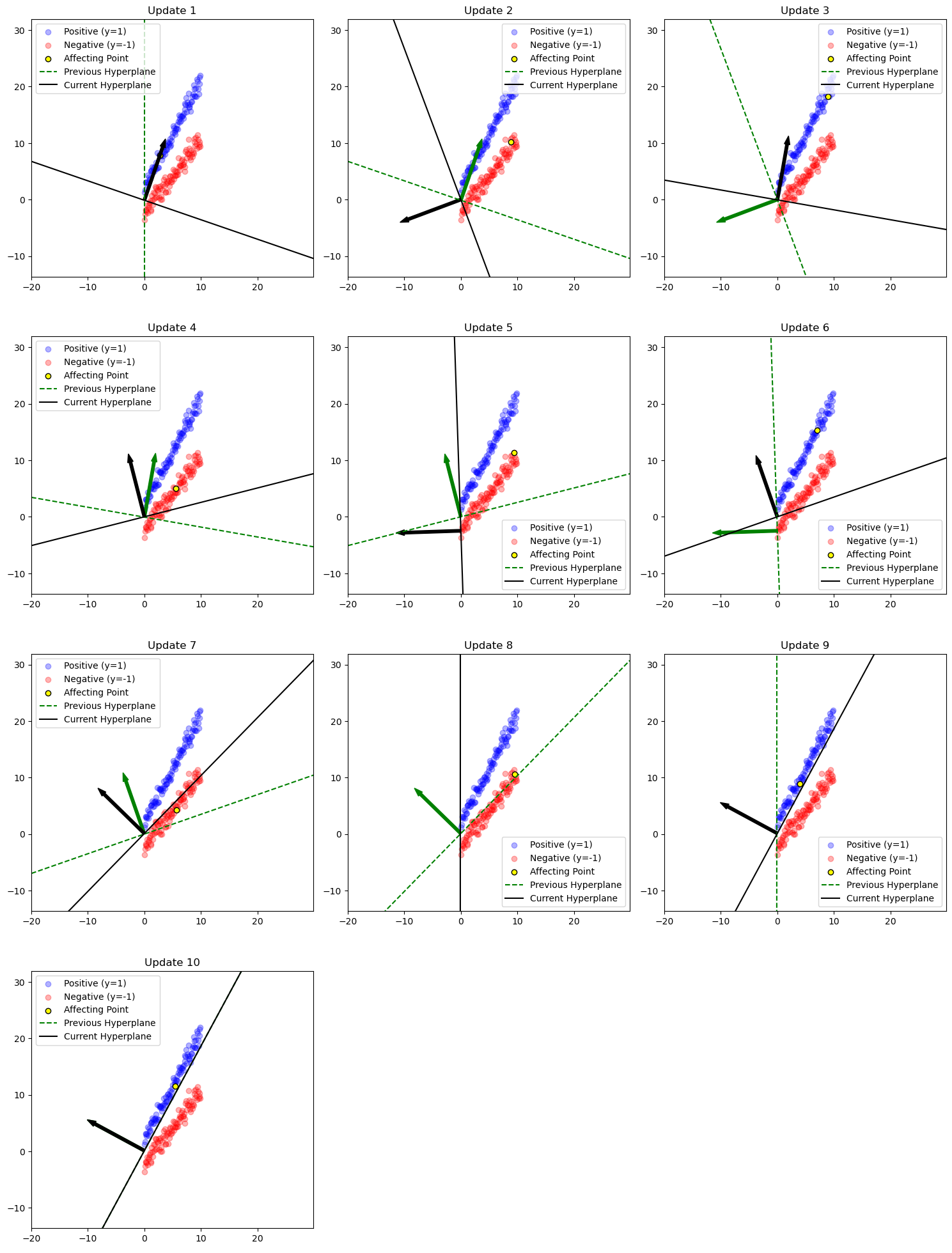
The following equation rewrites the hyperplane from its normal vector form into a slope-intercept form, which facilitates visualization.
$$ w_1 x_1 + w_2 x_2 + b = 0 \ $$$$ x_2 = -\frac{w_1 x_1 + b}{w_2} $$As illustrated in the figure below, this transformation makes it easier to observe how the hyperplane’s normal vector is influenced by the data points. The green arrow represents the normal vector before the update, while the black arrow shows the normal vector after the update.
For example, in Update 2, when a negative sample lies on positive side of the hyperplane, the green arrow shifts slightly away from this data point after the update, making it more likely for the point to appear on the opposite side in the direction of the updated normal vector. A more pronounced case can be seen in Update 4, where a negative sample (marked in yellow) initially lies on positive side of the hyperplane but moves to the opposite side following the update.
Show/Hide the code
| |
ML Components in Perceptron
In the case of perceptron, the hypothesis is the family of affine functions in $R^n$ the loss is the number of points misclassified by the perceptron. The optimizer is
$$ w \leftarrow w + y \cdot x \cdot \text{lr} $$$$ b \leftarrow b + y \cdot \text{lr} $$Week3
In the case of perceptron, the loss of one point is either 0 (correct prediction) or 1 (incorrect prediction) and the overall loss is the number of points that are incorrectly classified. This is a valid way to measure the approximation of the true unknown function $f$ by the hypothesis functions. Using different criteria to measure the deviation of hypothesis functions from the true function $f$ can lead to different final choice of $g$. For example, in a system designed to detect harmful content targeted at children, the probability of false negatives - that is, harmful content that goes undetected - should be minimized as much as possible. In this case, the evaluation criterion should prioritize penalizing false negatives to the greatest extent.
Logistic Regression
implementation of a logistic regression
Show/Hide the code
| |
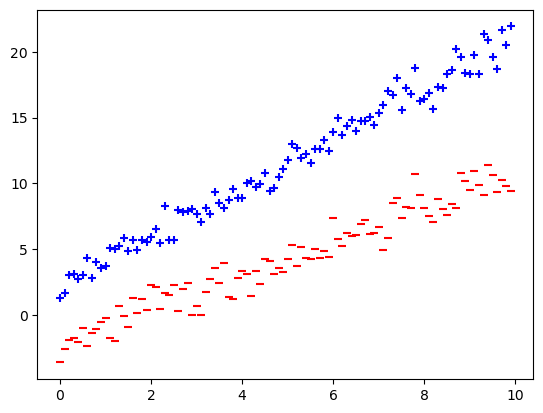
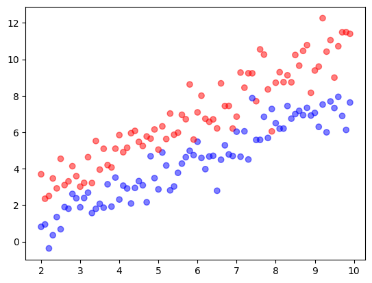
Try Logistic Regression on a Synthetic Dataset
generate data
Show/Hide the code
| |
learn
Show/Hide the code
| |
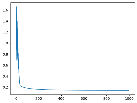
loss
Show/Hide the code
| |
visualize learning process
Show/Hide the code
| |
Try Logistic Regression on a Real Dataset
load data and learn
Show/Hide the code
| |
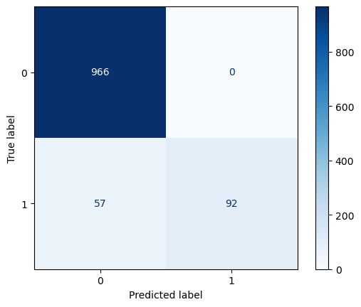
evaluate performance
Show/Hide the code
| |
Accuracy: 0.9488789237668162
Precision: 1.0
Recall: 0.6174496644295302
F1 Score: 0.7634854771784232

Classification Report:

              precision    recall  f1-score   support

         ham       0.94      1.00      0.97       966
        spam       1.00      0.62      0.76       149

    accuracy                           0.95      1115
   macro avg       0.97      0.81      0.87      1115
weighted avg       0.95      0.95      0.94      1115
Show/Hide the code
| |
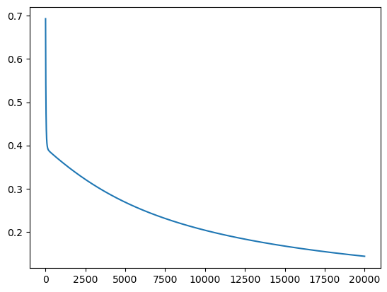
loss
Show/Hide the code
| |
Week 4
The loss for multi-output regression should be the sum of the losses for all outputs. Whether using MSE or other types of loss functions, it’s simply a numerical summation. However, since the outputs of classification tasks are interpreted as probabilities, their sum must be 1. This means that an increase in the probability of one class must lead to a decrease in the probabilities of other classes in order to maintain the total sum of 1.
As for the cross entropy loss, I prefer to view it from a probabilistic and statistical perspective, namely as minimizing the negative log-likelihood function.
For a binary classification task, define the random variable:
$$ X = \begin{cases} 1, & \text{if positive} \\ 0, & \text{if negative} \end{cases} $$Then $X \sim \text{Bern}(p)$, where $p$ is the probability of the sample being positive and $p$ is in effect a function of the model parameters $\mathbf{w}$
The probability mass function is:
$$ P(X=y) = p^y (1-p)^{1-y}, \quad y \in \{0,1\}. $$For a classification task with $K$ classes, let:
- $\mathbf{p} = (p_1, p_2, \dots, p_K)$ be the probability vector over all classes
- $\mathbf{y} = (y_1, y_2, \dots, y_K)$ be the one-hot encoded label
Then the probability of observing $\mathbf{y}$ is:
$$ P(\mathbf{X} = \mathbf{y}) = \prod_{k=1}^K{p_k^{y_k}}. $$The Maximum Likelihood Function for a multi-class classification problem with $n$ samples and $K$ possible classes is:
$$ L(\mathbf{y}|\mathbf{x}; \mathbf{p}) = \prod_{i=1}^n \prod_{k=1}^K p_{k}^{\,y_{k}}, $$where:
- $p_{i,k}$ is the predicted probability that sample $i$ belongs to class $k$, which is a function of the model parameters
- $y_{i,k}$ is the one-hot label
Taking the negative logarithm of the likelihood gives the negative log-likelihood:
$$ -\log L(\mathbf{y}|\mathbf{x}; \mathbf{p}) = -\sum_{i=1}^n \sum_{k=1}^K y_{k}\,\log p_{k}. $$Since only the true class has $y_{k}=1$, this simplifies to:
$$ -\log L(\mathbf{y}|\mathbf{x}; \mathbf{p}) = -\sum_{i=1}^n \log p_{i}, $$Week 5
- Input and output formats of the functions
The simplest form of Support Vector Machine (SVM), the Maximum Margin Classifier, shares the same family of hypotheses as the perceptron, namely a set of N-dimensional hyperplanes. The key difference lies in how they select the optimal hypothesis. The perceptron learning algorithm processes data points sequentially, one at a time. If a data point is misclassified, the algorithm updates the parameters, effectively adjusting the hypothesis.
By contrast, the Maximum Margin Classifier seeks an optimal hyperplane that maximizes the margin, positioning it as far as possible from all data points. SVMs take a N-dimensional vector as input which represents a data point. The output is predictions $\hat{y} \in {-1, 1}$
- Are they parametrized?
Yes, they are. the parameter space is $R^{(N+1)}$ where $N$ is the number of dimensions of input vectors.
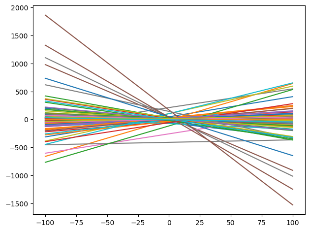
- Randomly sample 100 functions from this family
Suppose the dataset is 2-dimensional
Show/Hide the code
| |